Learning Statistics Using R: Role Type Classification: Case III (5 of 5)

Now we learn to create a labeled scatterplot using R. In labeled scatterplot we indicate different subgroups or categories within the data on the plot; by labeling each subgroup differently.

Note till now we were using "plot" or "scatter.smooth" function to create our scatter plot, but I have not found a nice and easy method of creating labeled scatterplot using these functions. So instead of these functions we will use another function from "car" package/library.

Recall the hot dog example from case I, in which 54 major hot dog brands were examined. In this study both the calorie content and the sodium level of each brand was recorded, as well as the type of hot dog: beef, poultry, and meat (mostly pork and beef, but up to 15% poultry meat). In this example we will explore the relationship between the sodium level and calorie content of hot dogs, and use the three different types of hot dogs to create a labeled scatterplot.
Lets do this with R using scatter.smooth function

# hotdog.txt is same as TA01_009.TXT
> hotdogdata <- read.table("hotdog.txt", sep="\t", header=T)
> attach(hotdogdata)
> names(hotdogdata)
[1] "HotDog"   "Calories" "Sodium"  
# lets try firt with scatter.smooth function.
# As of version R version 2.6.2 (2008-02-08), 'quanlity' argument
# does not result in a warning but newer version does; pointed out by Gabriele Righetti.
> png("/tmp/hotdogtry1.png", quality=100, width=480)
> scatter.smooth(Sodium, Calories)
# We try added label to this plot using text command/function.
# Bug-Fix: Gabriele Righetti
> text(Sodium,Calories, HotDog)
> dev.off()

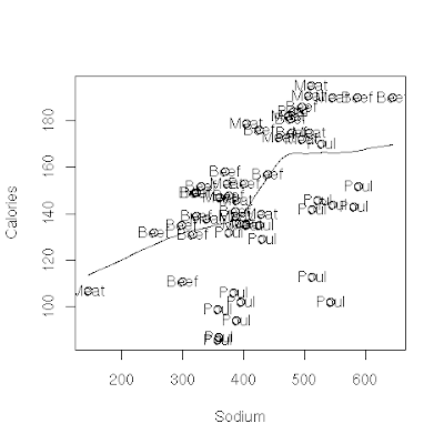
So here is our image, but this is not what we wanted. Here we have tried to add text/label to this using "text" function but it has become too ugly to look at. So now lets try creating a better labeled scatter plot using "car" library.
Lets do this with R using "car" library

# we already have data that is attached. so let first load the
# library.
> library("car")
> png("/tmp/hotdogtry2.png", quality=100, width=480)
> scatterplot(Calories ~ Sodium | HotDog)
> dev.off()

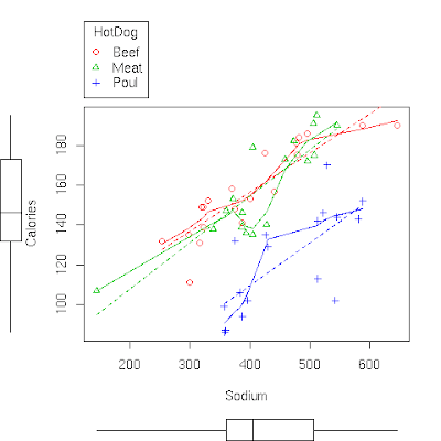
So this is out second graph and this looks much better than our earlier. Also there is an entire moive explaining concept of labeled scatterplot at the course website.

Lets Summarize:

• The relationship between two quantitative variables is visually displayed using the scatterplot, where each point represents an individual. We always plot the explanatory variable on the horizontal, X-axis, and the response variable on the vertical, Y-axis.
• When we explore a relationship using the scatterplot we should describe the overall pattern of the relationship and any deviations from that pattern. To describe the overall pattern consider the direction, form and strength of the relationship. Assessing the strength could be problematic.
• Adding labels to the scatterplot, indicating different groups or categories within the data, might help us get more insight about the relationship we are exploring.

Learning Statistics Using R: Role Type Classification: Case III (4 of 5)

To remind; we are learning to examine relationship between a response and a exaplanatory variable. In our case III both variables are quantitative (numerical).

We looked at the method to examine case III relationship between two quantitative variables in previous post. Lets understand it better with few more examples.

Example: The average gestation period, or time of pregnancy, of an animal is closely related to its longevity (the length of its lifespan.) Data on the average gestation period and longevity (in captivity) of 40 different species of animals have been examined, with the purpose of examining how the gestation period of an animal is related to (or can be predicted from) its longevity. (Reference: Rossman and Chance, Workshop Statistics. Discovery with Data and Minitab (2001). Original source: The 1993 World Almanac and Book of Facts).

The actual dataset for this example is available here and also as single zip file that includes all dataset of this site.
Lets examine this dataset using R:

# Lets read the dataset animals.dat into R.
# dataset is separated by a tab (\t) and header row 
# is present but not very intitutive so we will 
# change it later.

> animals <- read.table("animals.dat", sep="\t", header=TRUE)
# print names of the rows.
> names(animals)
[1] "animal"   "gestati3" "longevi4"
# we want to change "gestati3" and "logevi4"
> names(animals) <- c("animal", "gestation", "longevity")
> names(animals)
[1] "animal"    "gestation" "longevity"
# so assigning values to names() changes the names.
# now lets draw the scatterplot and examine the dataset.
# we want to create scatterplot in a png file for upload.
> png("/tmp/animal.png", quanlity=100, width=480)
> scatter.smooth(animals$long, main="Lifespan and Pregnancy", 
  xlab="Longevity (Years)", ylab="Gestation (Days)")
# following writes the graph to file. 
> dev.off()

• Direction: The direction of relationship is essentially positive, that is longer lifespan tends to have have longer times of pregnancy.
• Form: Again the form of relationship (between response and explanatory) variable is linear.
• Outliers: There seems to be one outlier at around 40 years. Lets use R to find out which observation is this?

  # we search for more than 35 year, just to be careful.
  > which(animals$longevity > 35)
  [1] 15
  # 'which' provides us with the observation number that has 
  # logevity > 35. Lets display that observation.
  # combination of which along with dataset give following:
  > animals [which(animals$longevity > 35), ]
       animal gestation longevity
  15 elephant       645        40
  

  
  So our outlier is an observation for elephant. Note that while this outlier definitely deviates from the rest of the data in term of its magnitude, it does follow the direction of the data.

Comments from course site: Another feature of the scatterplot that is worthwhile observing is how the variation in Gestation increases as Longevity increases. Note that gestation period for animal who live 5 years ranges from about 30 days up to about 120 days. On the other hand the gestation period of animals who live 12 years varies much more, and ranges from about 60 days and up to above 400 days.

Example: As another example, consider the relationship between the average fuel usage (in liters) for driving a fixed distance in a car (100 kilometers), and the speed at which the car drives (in kilometers per hour). (Reference: Moore and McCabe, Introduction to the Practice of Statistics, 2003. Original source: T.N. Lam "Estimating fuel consumption for engine size", Journal of transportation Engineering,111 (1985))

The actual dataset for this example is available here (See chapter 2) and also as single zip file that includes all dataset of this site.
Lets examine this dataset using R:

> sf <- read.table("speedfuel.txt", sep="\t", header=TRUE)
> png("/tmp/speedfuel.png", quanlity=100, width=480)
# check column names..
> scatter.smooth(sf$Speed, sf$Fuel, main="",   xlab="Speed (km/h)", 
  ylab="Fuel Used (liters/100km)")
> dev.off()

The data describe a relationship that decreases and then increases - the amount of fuel consumed decreases rapidly to a minimum for a car driving 60 kilometers per hour, and then increases gradually for speeds exceeding 60 kilometers per hour. This suggests that the speed at which a car economizes on fuel the most is about 60 km/h. This forms a curvilinear relationship which seems to be very strong, as the observations seem to perfectly fit the curve. Finally, there do not appear to be any outliers.

Example: Another example and scatterplot taken from course website provides a great opportunity for interpretation of the form of the relationship in context. The example examines how the percentage of participants who completed a survey is affected by the monetary incentive that researchers promised to participants. Here, is the scatterplot which displays the relationship: The positive relationship definitely makes sense in context, but what is the interpretation of the curvilinear form in the context of the problem? How can we explain (in context) the fact that the relationship seems at first to be increasing very rapidly, but then slows down?

Note that when the monetary incentive increases from $0 to $10, the percentage of returned surveys increases sharply - an increase of 27% (from 16% to 43%). However, the same increase of $10 from $30 to $40 doesn't show the same dramatic increase on the percentage of returned surveys - an increase of only 3% (from 54% to 57%). The form displays the phenomenon of "diminishing returns" - a return rate that after a certain point fails to increase proportionately to additional outlays of investment. $10 is worth more to people relative to $0 than to $30.

Learning Statistics Using R: Role Type Classification: Case III (3 of 5)

In next few posts we try to understand direction, form, strength and outliers of our Sign Legibility Distance Vs. Age scatterplot.

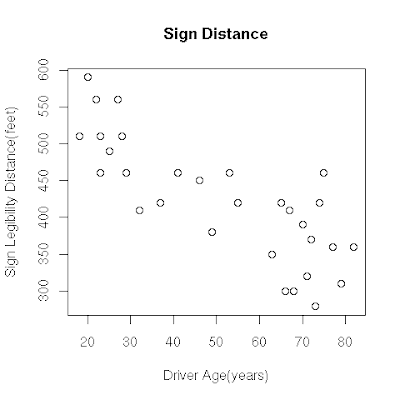
We try with simple scatterplot and then try to find its direction using R. So this is how our scatterplot looks when drawn using R.

# read the signdistance datafile that is included in here
# http://krishnadagli.blogspot.com/2008/07/learning-statistics-using-r-data-sets.html

> sigdist <- read.table("signdistance.txt", header=T, sep='\t')
# we want to create scatterplot in a png file, that is easy to upload.
> png("/tmp/signdist.png", quality=100, width=480)
> plot(sigdist, main="Sign Distance", xlab="Driver Age(years)", ylab="Sign Legibility Distance(feet)")
> dev.off()

So this how our scatterplot looks, we try to first find the direction of this plot.
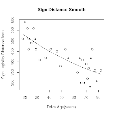
Find direction: (FIXME: Is this correct, what alternatives?): For finding direction of scatter plot we use one of R's function 'scatter.smooth'. The help page says that it plot and add a smooth curve computed by 'loess' to a scatter plot, and Wiki entry here mentions loess, or locally weighted scatterplot smoothing, as one of many "modern" modeling methods. Here is the R code to add a curve to our plot.

# we have already read data in sigdist object, lets use it.
# As we want to create and save the plot, we use png function.
>png("/tmp/sigdistsmooth.png", width=480, quality=100)
> scatter.smooth(sigdist, main="Sign Distance Smooth", 
  xlab="Drive Age(years)", ylab="Sign Legibility Distance(feet)")

Here is how our scatterplot along with a curve looks.
We can see that the direction of the relationship is negative, which makes sense in context since as you get older your eyesight weakens, and in particular older drivers tend to be able to read signs only at lesser distances. (How do we get an arrow drawn over the scatterplot just like its shown in the course?)

Find form: The form of the relationship seems to be linear. Notice how the points tend to be scattered about the line. Although, as we mentioned earlier, it is problematic to assess the strength without a numerical measure, the relationship appears to be moderately strong, as the data is fairly tightly scattered about the line. Finally, all the data points seem to "obey" the pattern- there do not appear to be any outliers.

Learning Statistics Using R: Role Type Classification: Case III (2 of 5)

As we have seen in our previous scatterplot, it is always the case that exaplanatory variable is plotted on horizontal, X-axis and response variable on Y-axis. If, at times we are not able to clearly identify explanatory and response variables then each of them can be plotted on either axis.

Interperting scatterplot: In our case-I we did comparative box plot and in case-II we did comparative bar plot/histogram but now how do we interpret scatterplot? What we dis is to describe the overall pattern of the distribution (of response variable) and any deviations (outliers) from that pattern, we take same approach for scatterplot. That is we describe overall pattern by looking at distribution's "Direction", "Form", and, "Strength" , and along with this we find outliers. Following from the course site puts it in a nice figure.


Lets discuss each of these three in details that describes overall pattern of relationship.

1. Direction: The direction of the relationship can be positive, negative, or neither. We identify the direction of relationship by looking at how scatterplot's points are moving along with x-y plane. Following figures shows example of positive, negative, and neither directions.
   • Positive direction: A positive (or increasing) relationship means that an increase in one of the variables is associated with an increase in the other.
     
   • Negative direction: A negative (or decreasing) relationship means that an increase in one of the variables is associated with a decrease in the other.
     
   • Neither: Not all relationships can be classified as either positive or negative.
2. Form: The form of the relationship is its general shape. When identifying the form, we try to find the simplest way to describe the shape of the scatterplot. There are many possible forms. Here are a couple that are quite common:
   • Linear Form: Relationships with a linear form are most simply described as points scattered about a line:
   • Curvilinear Form: Relationships with a curvilinear form are most simply described as points dispersed around the same curved line:
   • Other Forms: There are many other possible forms for the relationship between two quantitative variables, but linear and curvilinear forms are quite common and easy to identify. Another form-related pattern that we should be aware of is clusters in the data:
3. Strength: The strength of the relationship is determined by how closely the data follow the form of the relationship. Let's look, for example, at the following two scatterplots displaying a positive, linear relationship:
   The strength of the relationship is determined by how closely the data points follow the form. We can see that in the top scatterplot the the data points follow the linear patter quite closely. This is an example of a strong relationship. In the bottom scatterplot the points also follow the linear pattern but much less closely, and therefore we can say that the relationship is weaker. In general, though, assessing the strength of a relationship just by looking at the scatterplot is quite problematic, and we need a numerical measure to help us with that. We will discuss this later in this section.
4. Outliers: Data points that deviate from the pattern of the relationship are called outliers. We will see several examples of outliers during this section. Two outliers are illustrated in the scatterplot below:

Learning Statistics Using R: Role Type Classification: Case III (1 of 5)

Lets start with our next example; understanding relationship between two quantitative variables, ie. both explanatory and response variables are quantitative.

As in previous two cases we compared distribution of response variable with that of explanatory variables. To be specific, in case I we compared distribution of quantitative response with categorical explanatory variable and in case II we compared distribution of categorical response variable with categorical explanatory variable.
Now we have both variables as quantitative, more importantly we have a explanatory variable that is quantitiave. We will start understanding their relationship using "scatterplot".

We start with an example taken from course site.
A Pennsylvania research firm conducted a study in which 30 drivers (of ages 18 to 82 years old) were sampled and for each one the maximum distance at which he/she could read a newly designed sign was determined. The goal of this study was to explore the relationship between driver's age and the maximum distance at which signs were legible, and then use the study's findings to improve safety for older drivers. (Reference: Utts and Heckard, Mind on Statistics (2002). Originally source: Data collected by Last Resource, Inc, Bellfonte, PA.)

Since the purpose of this study is to explore the effect of age on maximum legibility distance,

• the explanatory variable is Age, and
• the response variable is Distance.

Here is what the raw data look like and its available here.
Note that the data structure is such that for each individual (in this case driver 1....driver 30) we have a pair of value (in this case representing the driver's age and distance). We can therefore think about this data as 30 pairs of values: (18,510), (32,410), (55,420)........(82,360).

The first step in exploring the relationship between driver age and sign legibility distance is to create an appropriate and informative graphical display. The appropriate graphical display for examining the relationship between two quantitative variables is the scatterplot.

Here is how a scatterplot is constructed for our example:

To create a scatterplot, each pair of values is plotted, so that the value of the explanatory variable (X) is plotted on the horizontal axis, and the value of the response variable (Y) is plotted on the vertical axis. In other words, each individual (driver, in our example) appears on the scatterplot as a single point whose x-coordinate is the value of the explanatory for that individual, and the y-coordinate is the value of the response. Following images taken from course website illustrate the same.

As we have data set, lets start doing the same using R.

# Read data using read.csv function, here separator is tab.
# Bug-Fix: Gabriele Righetti 
> signdist <- read.csv ("signdistance.txt", sep="\t", header=T)
> plot(signdist, type="b", main="Sign and Distance", col="blue", xlab="Driver Age", 
ylab="Sign Legibility Distance (Feet)")

The output of above simple command plot draws our scatter plot. Also note our scatter plot is different, that is we have lines along with points. That is possible with simple parameter "type=b" in plot commands. See the help page of plot command to see all types.
Another using "type=p" argument.

Learning Statistics Using R: Role Type Classification : Case II (2 of 2)

Following example from the course website provides an opportunity to analyze relationship between two categorical variables using R.

Study: An associated press article captured the attentions of readers with the headline "Night lights bad for kids?" The article was based on a 1999 study at the University of Pennsylvania and Children's Hospital of Philadelphia, in which parents were surveyed about the lighting conditions under which their children slept between birth and age 2 (lamp, night-light, or no light) and whether or not their children developed nearsightedness (myopia.) The purpose of the study was to explore the effect of a young child's night-time exposure to light on later nearsightedness.

The actual excel file can be downloaded from here. Or it can be downloaded as and csv file along with other data sets from here.

Lets try to do this analysis using R.

1. Find out explanatory and response variables:
   • Light:(No light/Night light/Lamp) this categorical variable is explanatory variable.
   • Nearsightedness: (Yes/No) this categorical variable is response variable since values (yes/no) depends on the value of Light variable.
   
   
2. Create a two-way summary table: Following steps shows how we summarize the data in a two-way table using R. Note there are multiple ways of creating two-way table in R but I have not successful at them.

    # Read data usingread.csv function.  
   > nightlight<-read.csv("nightlight.csv", header=T,sep=",")
   
   # Find row and column totals using addmargins function.
   > addmargins(table(nightlight),FUN=sum, quiet=F)
   Margins computed over dimensions
   in the following order:
   1: Light
   2: Nearsightedness
                Nearsightedness
   Light          No Yes sum
     lamp         34  41  75
     night light 153  79 232
     no light    155  17 172
     sum         342 137 479
   

   As we have seen earlier "table" command is used to tabulate data but we need row and column totals; that is possible using "addmargins" function. (I think this can also be achieved using combination of apply, t, cut and few other functions but I am not able to do so due to limited knowledge of R. Have a look at this discussion thread.)
   
   
3. Find percentage: As noted earlier, having sum does not help; we need to find percentage for comparing distribution of response variable.
   Again, as I am learning R I could not do this percentage calculation using combination of R commands but found a package (rather two) that does exactly what we want.
   
   • Using "CrossTable" function from library "gregmisc":
     

      # load the library 
     > library("gregmisc")
     Loading required package: gdata
     Loading required package: gmodels
     Loading required package: gplots
     Loading required package: gtools
     
     # Read data usingread.csv function.  
     > nightlight <- read.csv("nightlight.csv", header=T,sep=",")
     > CrossTable(table(nightlight), prop.t=FALSE, prop.c=FALSE, prop.r=TRUE, prop.chisq=F)
     
        Cell Contents
     |-------------------------|
     |                       N |
     |           N / Row Total |
     |-------------------------|
      
     Total Observations in Table:  479 
      
                  | Nearsightedness 
            Light |        No |       Yes | Row Total | 
     -------------|-----------|-----------|-----------|
             lamp |        34 |        41 |        75 | 
                  |     0.453 |     0.547 |     0.157 | 
     -------------|-----------|-----------|-----------|
      night light |       153 |        79 |       232 | 
                  |     0.659 |     0.341 |     0.484 | 
     -------------|-----------|-----------|-----------|
         no light |       155 |        17 |       172 | 
                  |     0.901 |     0.099 |     0.359 | 
     -------------|-----------|-----------|-----------|
     Column Total |       342 |       137 |       479 | 
     -------------|-----------|-----------|-----------|
     

     
     As we can see from the above output, "CrossTable" function provides us what we want. ( "prop.r=TRUE" provides us with row proportions.)
     
     
   • Using "Rcmdr" library
     This library provides nice GUI using which we can find row percentage and other details. Here is the screen shot of the same.
   
   
4. Interpret these results: Lets try to analyze these results. We want explore the effect of a young child's night-time exposure to light on later nearsightedness. From the above results lets note few things:
   • The results suggest that propotion of children 0.547 (or 54.7%) developed nearsightedness when exposed to lamp. This propotion is higher when we compare this to night light and no light propotion; that are 0.341 (or 34.1 %) and 0.099 (or 9.9 %) respectively.
   • That is there are 5 times higher chances of children developing nearsightedness when slept with lamp compared to children who slept without any lights.
   • Though 9.9 % of children developed nearsightedness when slept without any lights.

Learning Statistics Using R: Role Type Classification : Case II (1 of 2)

Case II of our role type classification includes study of relationship between a Categorical Explanatory and a Categorical Response variable.

We start with an example from the course web site to explore relationship between two categorical variables.
Example: In a survey, 1200 U.S. college students were asked about their body-image, underweight, overweight, or about right. We have to find answer to following questions:
If we had separated our sample of 1200 U.S. college students by gender and looked at males and females separately, would we have found a similar distribution across body-image categories?
More specifically,are men and women just as likely to think their weight is about right? Among those students who do not think their weight is about right, is there a difference between the genders in feelings about body-image?

So for answering these questions requires us to study the relationship between two categorical variables. Both response and explanatory variables are categorical since we want to find how gender (male/female) affects body image (underweight, overweight, right weight). Here in this study we have following:

• Gender: (Male/Female) as explanatory variable and it is a categorical variable.
• Body-image:(underweight, overweight, right weight) as response variable and it is a categorical variable.

As I could not find raw data for these example; we will directly use results derived at the course site instead of reading raw data in R and finding results.

To understand how body image is related to gender, we need an informative display that summarizes the data. In order to summarize the relationship between two categorical variables, we create a display called a two-way table.

Here is the two-way table for our example:

So our two-way table summarizes data of all 1200 students by gender and their body image as counts. The "Total" row or column is a summary of one of the two categorical variables, ignoring the other. In our example:

• The Total row gives the summary of the categorical variable Body-image:
  
• The Total column gives the summary of the categorical variable Gender:
  

Remember, though, that our primary goal is to explore how body image is related to gender. Exploring the relationship between two categorical variables (in this case Body-image and Gender) amounts to comparing the distributions of the response (in this case Body-image) across the different values of the explanatory (in this case males and females):
Note that it does not make sense to compare raw counts, because there are more females than males overall. So for example, it is not very informative to say "there are 560 females who responded 'About Right' compared to only 295 males," since the 560 females are out of a total of 760, and the 295 males are only out of a total of 440). We need to supplement our display, the two-way table, with some numerical summaries that will allow us to compare the distributions. These numerical summaries are found by simply converting the counts to percents within (or restricted to) each value of the explanatory variable separately! In our example: We look at each gender separately, and convert the counts to percents within that gender. Let's start with females:

Note that each count is converted to percents by dividing by the total number of females, 760. These numerical summaries are called conditional percents, since we find them by conditioning on one of the genders

Comments

1. In our example, we chose to organize the data with the explanatory variable Gender in rows and the response variable Body-image in columns, and thus our conditional percents were row percents, calculated within each row separately. Similarly, if the explanatory variable happens to sit in columns and the response variable in rows, our conditional percents will be column percents, calculated within each column separately.
2. Another way to visualize the conditional percents, instead of a table, is the double bar chart. This display is quite common in newspapers.

After looking at the numerical summary and graph lets try to put the results in words:

• The results suggest that propotion of males who are happy with their body image 'About right' is slightly less than among female student. That is 73.3 % of female students are happy with their body image compared to only 67 % of males.
• Female students who are not happy with their body image often feel they are overweight. That is 73.3 % are happy but remaining 21.4 % feel they are overweight compared to only 4.9 % feeling underweight.
• Male students who are not happy with their body image feel they are overweight about often as they feel they are underweight. That is 16.6 % student feel they are overweight while rougly same 16.2 % student feel they are underweight.

Learning Statistics Using R: Role Type Classification : Case I (1 of 1)

As we show earlier, Case I of our role type classification includes study of a relationship between a Categorical Explanatory and a Quantitative Response variable.

We start with an example from the course website.
Example:People who are concerned about their health may prefer hot dogs that are low in calories. A study was conducted by a concerned health group in which 54 major hot dog brands were examined, and their calorie contents recorded. In addition, each brand was classified by type: beef, poultry, and meat (mostly pork and beef, but up to 15% poultry meat).

The purpose of the study was to examine whether the number of calories a hot dog has is related to (or affected by) its type. (Reference: Moore, David S., and George P. McCabe (1989). Introduction to the Practice of Statistics. Original source: Consumer Reports, June 1986, pp. 366-367.) Answering this question requires us to examine the relationship between the categorical variable Type and the quantitative variable Calories. Because the question of interest is whether the type of hot dog affects calorie content,

• the explanatory variable is Type, and
• the response variable is Calories.

To explore how the number of calories is related to the type of hot dog, we need an informative visual display of the data that will compare the three types of hot dogs with respect to their calorie content. The visual display that we'll use is side-by-side boxplots. The side-by-side boxplots will allow us to compare the distribution of calorie counts within each category of the explanatory variable, hot dog type. We use R to do side-by-side box plot:

> hotdogdata <- read.csv ("TA01_009.TXT", header=T, sep="\t")
> attach(hotdogdata)
> boxplot(Calories[HotDog == 'Beef'], Calories[HotDog == 'Meat'], Calories[HotDog == 'Poul'], 
  border=c('blue', 'magenta','red'), 
  names=c('Beef','Meat', 'Poul'), 
  ylab='Calories', 
  main='Side By Side Comparative Boxplot of Calories')

Gabriele Righetti from Italy pointed out that it should be "names" and not "xlab" for naming boxplots. Thanks Gabriele.

The output of the above command displays a boxplot like following:
Lets also find five number summary for each type using R. Here is the output of the same:

> summary(Calories[HotDog=='Beef'])
   Min. 1st Qu.  Median    Mean 3rd Qu.    Max. 
  111.0   140.5   152.5   156.8   177.2   190.0 
> summary(Calories[HotDog=='Meat'])
   Min. 1st Qu.  Median    Mean 3rd Qu.    Max. 
  107.0   139.0   153.0   158.7   179.0   195.0 
> summary(Calories[HotDog=='Poul'])
   Min. 1st Qu.  Median    Mean 3rd Qu.    Max. 
   86.0   102.0   129.0   122.5   143.0   170.0 

Let's summarize the results we got and interpret them in the context of the question we posed: By examining the three side-by-side boxplots and the numerical summaries, we see at once that poultry hotdogs as a group contain fewer calories than beef or meat.
The median number of calories in poultry hotdogs (129) is less than the median (and even the first quartile) of either of the other two distributions (medians 152.5 and 153).
The spread of the three distributions is about the same, if IQR is considered (all slightly above 40), but the (full) ranges vary slightly more (beef: 79, meat:88, poultry 84). The general recommendation to the health conscious consumer is to eat poultry hotdogs.
It should be noted, though, that since each of the three types of hotdogs shows quite a large spread among brands, simply buying a poultry hotdog does not guarantee a low calorie food. What we learn from this example is that when exploring the relationship between a categorical explanatory variable and a quantitative response (Case I), we essentially compare the distributions of the quantitative response for each category of the explanatory variable using side-by-side boxplots supplemented by descriptive statistics.

So we can safely say, the relationship between a categorical explanatory and a quantitative response variable is summarized using:

• Data display: side-by-side boxplots
• Numerical summaries: descriptive statistics

That is we compare the distributions of the quantitative (response) variables for each category (of categorical variable or factors as in R).

Learning Statistics using R: Role-type classification (2 of 2)

Lets try few examples from the course web site. In these example we are presented with a brief description of a study involving two variables. We are required to determine which of the four cases represents the data sets of the problem. That is we need to identify if a variable is Categorical or Quantitative and which variable is Response and Explanatory variable.

1. A store asked 250 of its customers whether they were satisfied with the service or not. The purpose of this study was to examine the relationship between the customer's satisfaction and gender.
   
   In this example, Gender is explanatory variable and Statifaction based on gender is response variable. Both these variables are Categorical and hence this is an example of Case II.
   
   
2. A study was conducted in order to explore the relationship between the number of beers a person drinks, and his/her Blood Alcohol Level (in %).
   In this example; Both the explanatory (number of beers) and response (BAC) variables are quantitative in this case, and therefore this is an example of case III. Hence this is an example of case I.
   
   
3. A study was conducted in order to determine whether longevity (how long a person lives) is somehow related to the person's handedness (right-handed/left-handed).
   
   In this case the explanatory variable (handedness) is categorical and the response variables (longevity) is quantitative. This is, therefore an example of case I.

Learning Statistics using R: Data sets used in examples

The actual data is available from the course website but lately my links to actual data set is not working; perhaps those are changed? I am also not sure on how to upload these data sets on blogger. So I have uploaded a zip file containing all data sets at MegaShare. Here is the link to download file : http://www.MegaShare.com/497357 (Updated : 01-OCT-2008, size: ~5.2 K)

Learning Statistics using R: Role-type classification (1 of 2)

Most of the material here is taken from the course website!
The second module of the course explains the relationship between two variables. In earlier sections we learned how to work with a distribution of a single variable, either quantitative or categorical.
This section start with Role-Type classification of two variable:In most studies involving two variables, each of the variables has a role. We distinguish between:

• Response variable: the outcome of study.
• Explanatory varible: the variable that claims to explain, predict or affect the response.

The response variables are also known as "Dependent" variables and the explanatory variables as "Independent" variables. Dependent variable depend on the Independent variable and hence the name. A simple example would be of a function that computes the sum of passed arguments; in this case arguments (the values whose sum we need to find) are independent variables while output (sum of these values) is dependent variable.
Lets take 8 example from course website to make this clear. We will be using these examples for further variable type classification.

1. We want to explore whether the outcome of the study - the score on a test - is affected by the test-taker's gender. Therefore:
   • Gender is the explanatory variable
   • Test score is the response variable
2. How does the number of calories a hot dog has related to (or effected by) the type of hot dog (beef, meat or poultry)? (in other words, are there differences in the number of calories between the three type of hot dogs?)
   • Number of calories is response variable
   • Type of hot dog is explanatory variable
3. In this study we explore whether nearsightedness of a person can be explained by the type of light that person slept with as a baby. Therefore:
   • Light Type is the explanatory variable
   • Nearsightedness is the response variable
4. Are the smoking habits of a person (yes/no) related to the person's gender?
   • Gender of person (male/female) is explanatory variable
   • Smoking habit is response variable
5. Here we are examining whether a student's SAT score is a good predictor for the student's GPA in freshman year. Therefore:
   • SAT score is the explanatory variable
   • GPA of Freshman Year is the response variable
6. In an attempt to improve highway safety for older drivers, a government agency funded a research that explored the relationship between drivers' age and sign legibility distance (the maximum distance at which the driver can read a sign).
   • Driver's age is the explanatory variable
   • Sign legibility distance is response variable
7. Here we are examining whether a person's outcome on the driving test (pass/fail) can be explained by the length of time this person has practiced driving prior to the test. Therefore:
   • Time is the explanatory variable
   • Driving Test Outcome is the response variable
8. Can you predict a person's favorite type of music (Classical/Rock/Jazz) based on his/her IQ level?
   • IQ Level is explanatory variable
   • Type of music is response variable

Above examples helps in identifying response and explanatory variable but is it always clear what is the role classification? In other words, is it always clear which of the variables is the explanatory and which is the response?
Answer: NO! There are studies in which the role classification is not really clear. This mainly happens in cases when both variables are categorical or both are quantitative. An example could be a study that explores the relationship between the SAT Math and SAT Verbal scores. In cases like this, any classification choice would be fine (as long as it is consistent throughout the analysis).

We know that a variable is either categorical variable or quantitative variable. We use this information to further classify response and explanatory variables. With this role-type classification we get following 4 possibilities:

1. Case I: Explanatory is Categorical and Response is Quantitative variable.
2. Case II: Explanatory is Categorical and Response is Categorical variable.
3. Case III:Explanatory is Quantitative and Response is Quantitative variable.
4. Case IV: Explanatory is Quantitative and Response Categorical variable.

Following table taken from course web summarizes above 4 cases:
The couse warns us that this role-type classification serves as the infrastructure for the entire section. In each of the 4 cases, different statistical tools (displays and numerical measures) should be used in order to explore the relationship between the two variables.

Along with this course also suggest us following important rule:
Principle:
When confronted with a research question that involves exploring the relationship between two variables, the first and most crucial step is to determine which of the 4 cases represents the data structure of the problem. In other words, the first step should be classifying the two relevant variables according to their role and type, and only then can we determine the appropriate statistical tools.
Lets go back to our 8 examples and try to classify explanatory and response variables to categorical or quantitative variable.

1. We want to explore whether the outcome of the study - the score on a test - is affected by the test-taker's gender. Therefore:
   • Gender is the explanatory variable and it is categorical variable.
   • Test score is the response variable and it is quantitative variable.
   • Therefore this is an example of Case I.
2. How does the number of calories a hot dog has related to (or effected by) the type of hot dog (beef, meat or poultry)? (in other words, are there differences in the number of calories between the three type of hot dogs?)
   • Type of hot dog is explanatory variable and it is categorical variable.
   • Number of calories is response variable and it is quantitative variable.
   • Therefore this is an example of Case I.
3. In this study we explore whether nearsightedness of a person can be explained by the type of light that person slept with as a baby. Therefore:
   • Light Type is the explanatory variable and it is categorical variable.
   • Nearsightedness is the response variable and it is categorical variable.
   • Therefore this is an example of Case II.
4. Are the smoking habits of a person (yes/no) related to the person's gender?
   • Gender of person (male/female) is explanatory variable and it is categorical variable.
   • Smoking habit is response variable and it is categorical variable.
   • Therefore this is an example of Case II.
5. Here we are examining whether a student's SAT score is a good predictor for the student's GPA in freshman year. Therefore:
   • SAT score is the explanatory variable and it is quantitative variable.
   • GPA of Freshman Year is the response variable and it is quantitiative variable.
   • Therefore this is an example of Case III.
6. In an attempt to improve highway safety for older drivers, a government agency funded a research that explored the relationship between drivers' age and sign legibility distance (the maximum distance at which the driver can read a sign).
   • Driver's age is the explanatory variable and it is quantitiave variable.
   • Sign legibility distance is response variable and it is quantitative variable.
   • Therefore this is an example of Case III.
7. Here we are examining whether a person's outcome on the driving test (pass/fail) can be explained by the length of time this person has practiced driving prior to the test. Therefore:
   • Time is the explanatory variable and it is qunatitative variable.
   • Driving Test Outcome is the response variable and it is categorical variable.
   • Therefore this is an example of Case IV.
8. Can you predict a person's favorite type of music (Classical/Rock/Jazz) based on his/her IQ level?
   • IQ Level is explanatory variable and it is quantitiave variable.
   • Type of music is response variable and it is categorical variable.
   • Therefore this is an example of Case IV.

After this we learn more about role-type classification and which tool to use in which cases.

Learning Statistics using R: Rule Of Standard Deviation

Most of the material here is taken from the course website!
Following explains the rule of standard deviation, also known as The Empirical Rule. The rule is applied only to normal (symmetric) data distribution.

• Approximately 68% of the observations fall within 1 standard deviation of the mean.
• Approximately 95% of the observations fall within 2 standard deviations of the mean.
• Approximately 99.7% (or virtually all) of the observations fall within 3 standard deviations of the mean.

This rule provides more insights about standard deviation and following picture taken from course web site illustrates the same rule: Lets understand this with an example: The following data represents height data of 50 males. Lets use R to find 5 number summary of these and to confirm if the distribution is nomal - mound shaped.

# We use 'c' command to populate male vector; on which we will carry our operations.
male <- c(64, 66, 66, 67, 67, 67, 67, 68, 68, 68, 68, 68, 68, 69, 69, 69, 69, 69, 70, 70, 70, 70, 70, 70, 70, 71, 71, 71, 71, 71, 71, 71, 72, 72, 72, 72, 72, 72, 73, 73, 73, 74, 74, 74, 74, 74, 75, 76, 76, 77)
> hist(male)

In above code sample 'hist' command draws a histogram that has almost normal-mound shape. Here is the image that R draws for us. Lets find five number summary and confirm if standard deviation rule applies correctly to this data set.

# Just a simple summary command gives five point summary
> summary(male)
   Min. 1st Qu.  Median    Mean 3rd Qu.    Max. 
  64.00   68.25   70.50   70.58   72.00   77.00
> sd(male)
[1] 2.857786
# Lets apply first rule - 68% of data points are within (mean - 1 * SD) and (mean + 1 * SD)
> male >= (mean(male) - (1 * sd(male))) & male <= (mean(male) + (1 * sd(male)))
 [1] FALSE FALSE FALSE FALSE FALSE FALSE FALSE  TRUE  TRUE  TRUE  TRUE  TRUE
[13]  TRUE  TRUE  TRUE  TRUE  TRUE  TRUE  TRUE  TRUE  TRUE  TRUE  TRUE  TRUE
[25]  TRUE  TRUE  TRUE  TRUE  TRUE  TRUE  TRUE  TRUE  TRUE  TRUE  TRUE  TRUE
[37]  TRUE  TRUE  TRUE  TRUE  TRUE FALSE FALSE FALSE FALSE FALSE FALSE FALSE
[49] FALSE FALSE
# above command gives us the indices of male vector as TRUE where our condition satisfies.
# Lets count how many such obervations are there.
> length(male[male >= (mean(male) - (1 * sd(male))) & male <= (mean(male) + (1 * sd(male)))])
[1] 34
# So out of 50 observation 34 observation are with in mean +/- 1 SD. ie.
> 34/50 * 100
[1] 68
# So as rule suggests, 68% observations are with in mean +/- 1 SD.

# Lets check second rule - 95% of data points are within (mean - 2 * SD) and (mean + 2 * SD)
> length(male[male >= (mean(male) - (2 * sd(male))) & male <= (mean(male) + (2 * sd(male)))])
[1] 48
> 48/50 * 100
[1] 96
# So indeed 95% of data points are within mean +/- 2 SD.

# Lets check third rule - 99.7% of data points are within (mean - 3 * SD) and (mean + 3 * SD)
> length(male[male >= (mean(male) - (3 * sd(male))) & male <= (mean(male) + (3 * sd(male)))])
[1] 50
> 50/50*100
[1] 100
# this shows that 99.7% of data points are with in mean +/- 3 SD.

Following table taken from course website makes this more clear:
Summary:

• The standard deviation measures the spread by reporting a typical (average) distance between the data points and their average.
• It is appropriate to use the SD as a measure of spread with the mean as the measure of center.
• Since the mean and standard deviations are highly influenced by extreme observations, they should be used as numerical descriptions of the center and spread only for distributions that are roughly symmetric, and have no outliers.
• For symmetric mound-shaped distributions, the Standard Deviation Rule tells us what percentage of the observations falls within 1, 2, and 3 standard deviations of the mean, and thus provides another way to interpret the standard deviation's value for distributions of this type.

Learning Statistics using R: Standard Deviation and Histogram

Most of the material here is taken from the course website!
In following example we will see how histogram can help us to clarify the concept of Standard Deviation.
Example:
At the end of a statistics course, the 27 students in the class were asked to rate the instructor on a number scale of 1 to 9 (1 being "very poor", and 9 being "best instrctor I've ever had"). The following table provides three hypothetical rating data:
Following are the histogram of data of each class:
What can we say about standard deviation by looking at these histogram and data set?
Lets assume that the mean of all three data set is 5 (which is reasonable clear by looking at histograms) and we know (roughly) that standard deviation is average distance of all data points from their mean.

• For class I histogram most of the ratings are at 5 which is also the mean of the data set. So the average distance between mean and data points would be very small (since most of the data points are at mean).
• For class II histogram most of the ratings are at far points from mean - 5. In this case most of the data points are at two extrems at 1 and 9. So the average distance between mean and data points would be larger.
• For class III histgram data points are evenly distributed around mean. We can safely say that in this case the average distance between mean and data points would be greater than that of class I but smaller than that of class II. ie. in-between class I and class II standard deviation.

Lets check our assumption by loading these data set into R and verifying standard deviation of each. The excel contained data set can be downloaded from here.

> class1 <- c(1,1,5,5,5,5,5,5,5,5,5,5,5,5,5,5,5,5,5,5,5,5,5,5,5,9,9)
> sd(class1)
[1] 1.568929
> summary(class1)
   Min. 1st Qu.  Median    Mean 3rd Qu.    Max. 
      1       5       5       5       5       9 

> class2 <- c(1,1,1,1,1,1,1,1,1,1,1,1,1,5,9,9,9,9,9,9,9,9,9,9,9,9,9)
> sd(class2)
[1] 4
> summary(class2)
   Min. 1st Qu.  Median    Mean 3rd Qu.    Max. 
      1       1       5       5       9       9 

> class3 <- c(1,2,3,4,5,6,7,8,9,1,2,3,4,5,6,7,8,9,1,2,3,4,5,6,7,8,9)
> sd(class3)
[1] 2.631174
> summary(class3)
   Min. 1st Qu.  Median    Mean 3rd Qu.    Max. 
      1       3       5       5       7       9 

So we have following standard deviation for our 3 class ratings

• Class I : 1.568929
• Class II : 4.0
• Class III : 2.631174

(Note that excel may vary a bit in results of standard deviation if you are using stdev function.) So calculated standard deviation confirm our assumption that we made by looking at histograms.

Learning Statistics using R: Standard Deviation

Most of the material here is taken from the course website!
Earlier we examined measure of spread using Range(max - min) and IQR(the range covered by middle 50% data). We also noted that IQR should be used when median is used as measure of center. Now we move to another measure of spread called standard deviation.

The idea behind standard deviation is to quantify the spread of distribution by measuring how far the observations are from mean of distribution. That is how distant observations are located from the mean of all observations. The standard deviation gives average (or typical distance) between an observation/data point and the mean, X-bar.

Lets understand standard deviation using an example; we calculate standard deviation step by step using R commands. (There is a single R function to do the same!)
Assume we have following data set of 8 observations:
7, 9, 5, 13, 3, 11, 15, 9

• Calculate mean:
  We use R's 'c' function to combine them in a vector and then use mean function to calculate mean of the data set.

  > dataset <- c(7, 9, 5, 13, 3, 11, 15, 9)
  > is.vector(dataset)
  [1] TRUE
  # we have stored our observation in a vector called dataset
  > mean(dataset)
  [1] 9
  # so we have 9 as the mean of our data set; now we need to find
  # distance of each observation from this value : 9.
  > deviation <- c (dataset - 9)
  > deviation
  [1] -2  0 -4  4 -6  2  6  0
  # above command directly gives us deviation of each observation from 
  # the mean; that we have stored in another vector called deviation.
  

  Thinking about the idea behind the standard deviation being an average (typical) distance between the data points and their mean, it will make sense to average the deviations we got. Note, however, that the sum of the deviations from the mean is always 0.
  
  
• Square of deviation:
  So we square each of the deviation and then take its average; which following R code does:
  

  # we can use either of following two methods to calculate square of
  # deviations.
  > deviation ^ 2
  [1]  4  0 16 16 36  4 36  0
  
  > deviation * deviation
  [1]  4  0 16 16 36  4 36  0
  

• Average the square deviations by adding them up, and dividing by n-1, (one less than the sample size): Lets do that in R.

  > (sum(deviation ^ 2)) / (length(dataset) - 1)
  [1] 16
  

  This average of the squared deviations is called the variance of the data.
  
  
• Find standard deviation:
  The standard deviation of the data is the square root of the variance. So in our case it would be square root of 16.

  >sqrt(16)
  [1] 4
  

  Why do we take the square root? Note that 16 is an average of the squared deviations, and therfore has different units of measurement. In this case 16 is measured in "squared deviation", which obviously cannot be interpreted. We therefore, take the square root in order to compensate for the fact that we squared our deviations, and in order to go back to the original units of measurement.

Properties of the Standard Deviation:

1. It should be clear from the discussion thus far that the standard deviation should be paired as a measure of spread with the mean as a measure of center.
2. Note that the only way, mathematically, in which the standard deviation = 0, is when all the observations have the same value. Indeed in this case not only the standard deviation is 0, but also the range and the IQR are 0.
3. Like the mean, the SD is strongly influenced by outliers in the data. Consider our last example: 3, 5, 7, 9, 9, 11, 13, 15 (data ordered). If the largest observation was wrongly recorded as 150, then: the average would jump up to 25.9, and the standard deviation jumps up to 50.3 Note that in this simple example it is easy to see that while the standard is strongly influenced by outliers, the IQR is not! In both cases, the IQR will be the same since, like the median, the calculation of the quartiles depends only on the order of the data rather than the actual values.

Choosing Numerical Summaries

• Use mean and the standard deviation as measures of center and spread only for reasonably symmetric distributions with no outliers.
• Use the five-number summary (which gives the median, IQR and range) for all other cases.

R function for Standard Deviation: There is a single R function "sd" that calculates Standard Deviation of dataset, just be careful to use "na.rm=TRUE" argument if you have NA values in your dataset. This function would return vector of SD of columns if dataset is dataframe or matrix. Remember its column's SD and not rows by default.

Learning Statistics using R: Five Number Summary

Most of the material here is taken from the course website!
Before we go ahead and learn how graphical representation of Five Number Summary, let check out few intersting course problems.
Here they are:

1. Example 1: A survey taken of 140 sports fans asked the question: "What is the most you have ever spent for a ticket to a sporting event?"
   The five-number summary for the data collected is:
   min = 85 Q1 =130 median = 145 Q3 = 150 max = 250
   Should the smallest observation be classified as an outlier?
2. Example 2: A survey taken in a large statistics class contained the question: "What's the fastest you have driven a car (in mph)?"
   The five-number summary for the 87 males surveyed is:
   min=55 Q1=95 Median=110 Q3=120 Max=155
   Should the largest observation in this data set be classified as an outlier?

Important Summary About Spread

• The range covered by the data is the most intuitive measure of spread and is exactly the distance between the smallest data point - min and the largest one - Max.
• Another measure of spread is the inter-quartile range (IQR) which is the range covered by the middle 50% of the data.
• IQR = Q3-Q1, the difference between the third and first quartiles. The first quartile (Q1) is the value such that one quarter (25%) of the data points fall below it. The third quartile is the value such that three quarters (75%) of the data points fall below it.
• The IQR should be used as a measure of spread of a distribution only when the median is used as a measure of center.
• The IQR can be used to detect outliers using the 1.5 * IQR (1.5 times IQR) criterion.

Five Number Summary: So far, in our discussion about measures of spread, the key players were:

• The extremes (min and Max) which provide the range covered by all the data, and
• The quartiles (Q1, M and Q3), which together provide the IQR, the range covered by the middle 50% of the data.

The combination of all five numbers (min, Q1, M, Q3, Max) is called the five number summary, and provides a quick numerical description of both the center and spread of a distribution.
Boxplot can be used for graphically summarizing these five number summary of the distribution of a quantitative. Lets start doing boxplots in R.

Example: Best Actor Oscar Winners:
This time we use best actor Oscar winners instead of actress and draw a boxplot using R.

# read the actor.csv file.
>actor<-read.csv("actor.csv", header=T, sep=",")
> attach(actor)
>boxplot(Age, border=c('blue'), xlab='Actor Age')

Here is how our boxplot of actor data set looks:
The boxplot graphically represents the distribution of a quantitative variable by visually displaying the five number summary and any observation that was classified as a suspected outlier using the 1.5(IQR) criterion.

Example: Best Actress Oscar Winners:
We use our actress data set again to draw another box plot:

# read the actress.csv file.
>actress<-read.csv("actress.csv", header=T, sep=",")
> attach(actress)
> boxplot(Age, border=c('magenta'), xlab='Actress Age')

Here is how our actress box plot looks drawn using R: Following graph taken from the course website highlights various details of boxplot done for actress data set. There are couple of interactive examples of boxplot at course website, try doing them.

Example: Best Actress and Actor Oscar Winners: Side by Side Comparative Boxplots. So far we have examined the age distributions of Oscar winners for males and females separately. It will be interesting to compare the age distributions of actors and actresses who won the best acting Oscar. To do that we will look at side-by-side boxplots of the age distributions by gender.
Its quite easy to do side by side boxplots in R. Following code shows how to do it:

# read the actor.csv file.
>actor <-read.csv("actor.csv", header=T, sep=",")
>actress <-read.csv("actress.csv", header=T, sep=",")
# Following is one single command 
# Bug-Fix: Gabriele Righetti 
> boxplot(actor$Age, actress$Age, border=c('blue','magenta'), names=c('Actor','Actress'), ylab='Age',main='Side-By-Side (Comparative) Boxplots\nAge of Best Actor/Actress Winners (1970-2001)')
>

This is how our final output from R look:
Recall also that we found the five-number summary and means for both distributions:

• Actors: min=31, Q1=37.25, M=42.5, Q3=50.25, Max=76
• Actresses: min=21, Q1=32, M=35, Q3=41.5, Max 80

Based on the graph and numerical measures, we can make the following comparison between the two distributions:

• Center: The graph reveals that the age distribution of the males is higher than the females' age distribution. This is supported by the numerical measures. The median age for females (35) is lower than for the males (42.5). Actually, it should be noted that even the third quartile of the females' distribution (41.5) is lower than the median age for males. We therefore conclude that in general, actresses win the Best Actress Oscar at a younger age than the actors do.
• Spread: Judging by the range of the data, there is much more variability in the females' distribution (range=59) than there is in the males' distribution (range=35). On the other hand, if we look at the IQR, which measures the variability only among the middle 50% of the distribution, we see more spread among males (IQR=13) than the females (IQR=9.5). We conclude that among all the winners, the actors' ages are more alike than the actresses' ages. However, the middle 50% of the age distribution of actresses is more homogeneous than the actors' age distribution.
• Outliers: We see that we have outliers in both distributions. There is only one high outlier in the actors' distribution (76, Henry Fonda, On Golden Pond), compared with three high outliers in the actresses' distribution.

Send Your Name to the Moon

NASA invites people of all ages to join the lunar exploration journey with an opportunity to send their names to the moon aboard the Lunar Reconnaissance Orbiter, or LRO, spacecraft.

Here is my certificate of participation!

Learning Statistics using R:Detecting Outliers with IQR

Most of the material here is taken from the course website!
An Outlier is an observation/data-point in set of observations (data set) that is far removed in values from other observations. An outlier is either very large or very small value and as noted earlier affects the mean of the data set. More about Outlier is here.

The (1.5 * IQR) criteria for finding outliers (1.5 times IQR):
An observation is suspected outliers if it is:

1. Below Q1 - (1.5 * IQR): that is Q1 minus 1.5 times IQR.
2. Above Q3 + (1.5 * IQR): that is Q2 minus 1.5 times IQR.

The following picture illustrates the 1.5 * IQR rule:
Example: Best Actress Oscar Winners:
We continue with our Best Actress Oscar winner data set. Here we will try to locate names of actress whose age is beyond the 1.5 * IQR range.

# we have data in 'actress' data frame; just check the quantile
> quantile(Age, names=T)   
0%   25%   50%   75%  100% 
21.00 32.50 35.00 41.25 80.00 

# Lets check the IQR 
> IQR(Age)
[1] 8.75

# Now lets see how to retrieve value for Q1 - First quantile
> quantile(Age,0.25) 
25% 32.5

# (Is this correct method?)
# As can be seen above passing a value 0.25 returns value of the first quantile. 
# now lets see what is the value for Q1 - (1.5 * IQR)
>quantile(Age, 0.25) - (IQR(Age) * 1.5) 
  25% 19.375
# Okay so this also works!

# now how do we get names of all actress whose age is less than 19.375?
>which(Age < (quantile(Age, 0.25) - IQR(Age) * 1.5))
integer(0)
# So in our data set there is no actress whose age is less than 19.375 since the smallest is of age 21!

# now lets try to find upper/higher suspected outliers. 
# Remember its Q3 + (IQR * 1.5)
>quantile(Age,0.75) + (IQR(Age) * 1.5) 
  75% 
54.375

# Okay so far so good; lets get age that are greater than 54.375
> Age > quantile(Age,0.75) + (IQR(Age) * 1.5 ) 
[1] FALSE FALSE FALSE FALSE FALSE FALSE FALSE FALSE FALSE FALSE FALSE  TRUE
[13] FALSE FALSE FALSE  TRUE FALSE FALSE FALSE  TRUE FALSE FALSE FALSE FALSE
[25] FALSE FALSE FALSE FALSE FALSE FALSE FALSE FALSE

# See it returns TRUE in the indices where our condition matches.

> which(Age > quantile(Age,0.75) + (IQR(Age) * 1.5 ))
[1] 12 16 20
# which command returns the same but actual index number; but how do we get names?

> actress[which(Age > quantile(Age,0.75) + (IQR(Age) * 1.5 )),]   
    Year      Name                   Movie              Age
12 1981   Kathryn Hepburn    On Golden Pond             74
16 1985   Geraldine Page     A Trip to the Bountiful    61
20 1989   Jessica Tandy      Driving Miss Daisy         80

# so the comma (,) at the end does the trick. Lets try to do without "which" command.


>actress[ Age > (quantile(Age,.75, names=T) + (IQR(Age) * 1.5)),]  
    Year      Name                   Movie              Age
12 1981   Kathryn Hepburn    On Golden Pond             74
16 1985   Geraldine Page     A Trip to the Bountiful    61
20 1989   Jessica Tandy      Driving Miss Daisy         80

# so finally we got suspected outliers!

Other methods:
We can draw boxplot to visually detect outliers. (But following does not seem that helpful?)

> boxplot(Age)
# or
> plot(lm(Age ~ 1))
# or using library car
> library("car")
> outlier.test(lm(Age ~ 1))

max|rstudent| = 3.943262, degrees of freedom = 30,
unadjusted p = 0.0004461754, Bonferroni p = 0.01427761

Observation: 20